Excel: Summary from different sheets

Description: Pivot table wizard can be used for merging the data from different sheets.
Steps:
1. Select PivotTable and PivotChart Wizard option.
[Normally this option is not available in menu. Add this from Office icon-> Excel Options->Customize->All Commands-> PivotTable and PivotChart Wizard]


2. Select “Multiple consolidation ranges” and click next.

3. Select “Create a single page field for me” and click Next

4. Add ranges from different sheets and click Next

5. Specify whether the summary is needed in existing sheet or in new sheet and click Finish

We have more Pivot options under PivotTable Tools -> Options tab.

Excel: Table

Description: Insert table is a new feature in Excel 2007. Even though we can form tables using columns, rows and Gridlines in Excel, Insert table option is having lot of advantages or features in it.

Steps for inserting a table:
      1. Select the cells/ columns required to be part of the table.
      2. Click Insert-> Table option.
      3. Specify whether your table is having headers or not.
We have lot of formatting options for the table as given below



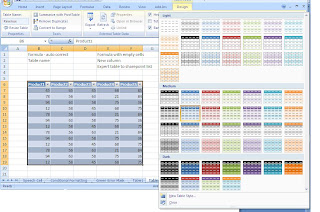
We have more options under Table Tools -> Design tab. Some of the features are export the table to SharePoint list/Visio pivot diagram, Summarize with Pivot table, Convert to Range, etc.
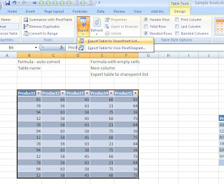
Main features of Table are given below.
Inclusion of new columns or Rows
When you add a new column near to the table, it automatically format and include the column to the table. Same way, it will format the new rows too.
Formulas
Table will take care of the empty cells referred in formulas. When you add a new record/row into the table, it automatically modifies the formulas which refer to the columns of the table.
Table Name
We can name the table using Table design tab.

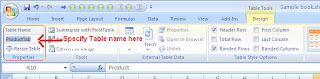
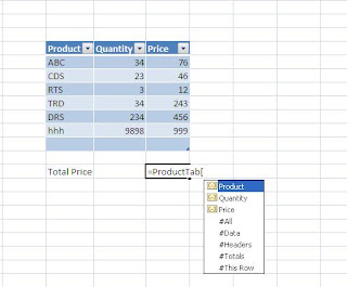
By default system will name each table as Table1, Table2, and so on. Table names are useful to create formulas in a more meaningful way. We can refer the table from any sheet using the table name. Also, each column names are getting intellisence as follows.
Here, Product Tab, ProductTab11 are table names.

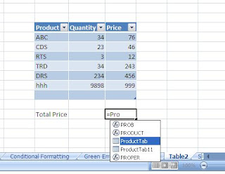
Column names are also getting intellisense as follows.

Freeze heading
Freeze the top row or portions of excel, to refer the column headings when you scroll down. If we have multiple tables/ headings, then the freeze feature will not be helpful. For avoiding this limitation, Table feature is came with an excellent feature, while scrolling the table change the real column heading [A, B, C,..] with column name of the Table.

Note: this will be available, only when you point to the table.

Excel: Green Error Mask

Description: This is the familiar green mark appearing in the left top corner of the cell. It indicates that, the data present in the cell is having some discrepancy or error. It is up to the user to correct the errors.

Number Stored As Text
One such indication is number is stored as Text. If a number stored in text format, this data will not be considered for any formulas referring the cell; in turn gives wrong data or result.

For avoiding this error, click on the cell and select the icon appearing on the left side of the cell
For Selecting all such errors in the sheet and act on it, press Ctrl+A two times. Click on one cell contains the error mask, press ctrl+A twice for selecting the entire sheet. Then the icon will appear on the top left corner of the sheet.


Inconsistent Formula
This error mark represent the cell is having a formula which is different from the adjacent cells. In the below screen shot, we used the formula as Amount*3.2% in all cells except the one with green error mask, where we used the formula Amount*3.3%.

Formula Omits Adjacent Cells
This indicates that the formula is omitted some data adjacent to it. In the below example, we calculated the Total revenue as a sum of revenues from Jan to April. After that, we added the revenue of May.

Excel: Conditional Formatting

Description: Make the business data more appealing using color or icon combinations. Old versions of Excel are having a limitation of maximum 3 conditions. In Excel 2007, we can have more conditions. Different options available are:-

Data Bars – Represent the data along with a graphical notation of the data.
Color Scales – Represent the value using color ranges
Icon Sets: - suitable for specific range of values like grades, ranks, etc.
Top/Bottom Rules: - Useful when we want to highlight Top 10 values or bottom 10% items or the items above/below average.
Highlight Cells Rule: - Useful when we need to apply the style using complex conditions.

Excel : Paste Special

Description: Paste Special feature is having lot of inner features. In this session, let us look into few of them.

Skip Blanks
Consider the scenario where a salesman, who needs to travel across the country, wants to fill his attendance. He filled the details in the following format

Now he wants to merge these two sheets. Here, we can use the skip blank feature of paste special.

Steps:
1. Copy the Attendance details from one table.
2. Point in the first cell [first cell of the column, which needs to be merged] of the second table.
3. Right click and select Paste Special
4. Check the Skip blanks option
5. Click OK.

Result:

Math
Consider the scenario, where we want to change the price to 3.5% of the existing Price. Place the modified Price data in the Price column itself.

Steps:
1. Place 3.5 in a cell.
2. Copy the value
3. Point the first cell of the Price column
4. Right click and Select Paste Special
5. Select Multiply option under Operation
6. Click OK



Note: Use Add for adding a single value to the entire column, Divide for dividing the column data with a single value and Subtract for deducting particular value from column data.
Paste Special is also giving the options for Pasting only the Column Widths, Values, Formats, etc.

Source Width
Description: Copy data from one location to another will change the format, column widths, etc. For keeping the source data column width follow the steps below.

Steps:
1. Copy data/cells
2. Paste to the destination
3. Click on the Smart Tag appeared.



4. Options available are
• Keep Source Formatting
• Use destination Theme
• Match destination formatting
• values and Number formatting
• Keep Source Column Widths
• Formatting Only
• Link Cells
5. Select ‘Keep Source Column Widths’ option.